A Comprehensive Guide to Data Exploration
Overview
- A complete tutorial on data exploration (EDA)
- We cover several data exploration aspects, including missing value imputation, outlier removal, and the art of feature engineering
Introduction
I can confidently say this because I’ve been through such situations, a lot.
1. Steps of Data Exploration and Preparation
Remember the quality of your inputs decide the quality of your output. So, once you have got your business hypothesis ready, it makes sense to spend lot of time and efforts here. With my personal estimate, data exploration, cleaning and preparation can take up to 70% of your total project time.
Below are the steps involved to understand, clean and prepare your data for building your predictive model:
- Variable Identification
- Univariate Analysis
- Bi-variate Analysis
- Missing values treatment
- Outlier treatment
- Variable transformation
- Variable creation
Finally, we will need to iterate over steps 4 – 7 multiple times before we come up with our refined model.
Let’s now study each stage in detail:-
Variable Identification
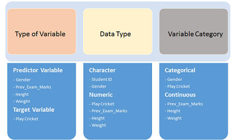
First, identify Predictor (Input) and Target (output) variables. Next, identify the data type and category of the variables.
Let’s understand this step more clearly by taking an example.
Example:- Suppose, we want to predict, whether the students will play cricket or not (refer to the data set). Here you need to identify predictor variables, target variables, the data type of variables, and the category of variables.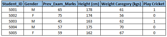 Below, the variables have been defined in a different categories:
Univariate Analysis
At this stage, we explore variables one by one. The method to perform univariate analysis will depend on whether the variable type is categorical or continuous. Let’s look at these methods and statistical measures for categorical and continuous variables individually:
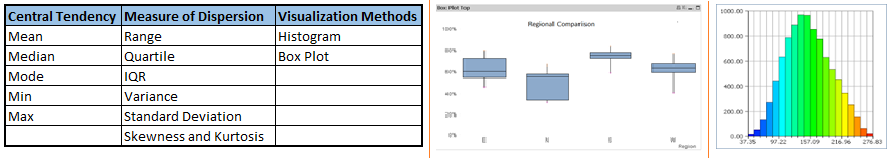
Continuous Variables:- In the case of continuous variables, we need to understand the central tendency and spread of the variable. These are measured using various statistical metrics visualization methods as shown below:
 Note: Univariate analysis is also used to highlight missing and outlier values. In the upcoming part of this series, we will look at methods to handle missing and outlier values. To know more about these methods, you can refer course descriptive statistics from Udacity.
Categorical Variables:- For categorical variables, we’ll use frequency table to understand distribution of each category. We can also read as percentage of values under each category. It can be be measured using two metrics, Count and Count% against each category. Bar chart can be used as visualization.
Bi-variate Analysis
Bi-variate Analysis finds out the relationship between two variables. Here, we look for association and disassociation between variables at a pre-defined significance level. We can perform bi-variate analysis for any combination of categorical and continuous variables. The combination can be: Categorical & Categorical, Categorical & Continuous and Continuous & Continuous. Different methods are used to tackle these combinations during analysis process.
Let’s understand the possible combinations in detail:
Continuous & Continuous: While doing bi-variate analysis between two continuous variables, we should look at scatter plot. It is a nifty way to find out the relationship between two variables. The pattern of scatter plot indicates the relationship between variables. The relationship can be linear or non-linear.
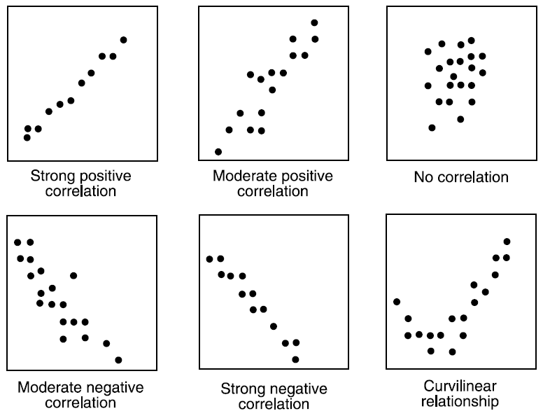 Scatter plot shows the relationship between two variable but does not indicates the strength of relationship amongst them. To find the strength of the relationship, we use Correlation. Correlation varies between -1 and +1.
Correlation can be derived using following formula:
Correlation = Covariance(X,Y) / SQRT( Var(X)* Var(Y))
Various tools have function or functionality to identify correlation between variables. In Excel, function CORREL() is used to return the correlation between two variables and SAS uses procedure PROC CORR to identify the correlation. These function returns Pearson Correlation value to identify the relationship between two variables:
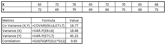
In above example, we have good positive relationship(0.65) between two variables X and Y.
Categorical & Categorical: To find the relationship between two categorical variables, we can use following methods:
- Two-way table: We can start analyzing the relationship by creating a two-way table of count and count%. The rows represents the category of one variable and the columns represent the categories of the other variable. We show count or count% of observations available in each combination of row and column categories.
- Stacked Column Chart: This method is more of a visual form of Two-way table.
- Chi-Square Test: This test is used to derive the statistical significance of relationship between the variables. Also, it tests whether the evidence in the sample is strong enough to generalize that the relationship for a larger population as well. Chi-square is based on the difference between the expected and observed frequencies in one or more categories in the two-way table. It returns probability for the computed chi-square distribution with the degree of freedom.
Probability of 0: It indicates that both categorical variable are dependent
Probability of 1: It shows that both variables are independent.
Probability less than 0.05: It indicates that the relationship between the variables is significant at 95% confidence. The chi-square test statistic for a test of independence of two categorical variables is found by:
![]() where O represents the observed frequency. E is the expected frequency under the null hypothesis and computed by:
where O represents the observed frequency. E is the expected frequency under the null hypothesis and computed by:![]()
From previous two-way table, the expected count for product category 1 to be of small size is 0.22. It is derived by taking the row total for Size (9) times the column total for Product category (2) then dividing by the sample size (81). This is procedure is conducted for each cell. Statistical Measures used to analyze the power of relationship are:
- Cramer’s V for Nominal Categorical Variable
- Mantel-Haenszed Chi-Square for ordinal categorical variable.
Different data science language and tools have specific methods to perform chi-square test. In SAS, we can use Chisq as an option with Proc freq to perform this test.
Categorical & Continuous: While exploring relation between categorical and continuous variables, we can draw box plots for each level of categorical variables. If levels are small in number, it will not show the statistical significance. To look at the statistical significance we can perform Z-test, T-test or ANOVA.
- Z-Test/ T-Test:- Either test assess whether mean of two groups are statistically different from each other or not.
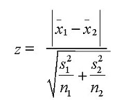 If the probability of Z is small then the difference of two averages is more significant. The T-test is very similar to Z-test but it is used when number of observation for both categories is less than 30.
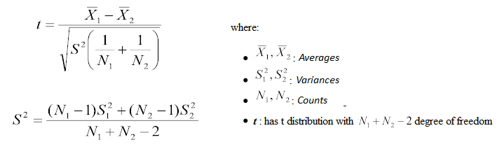
- ANOVA:- It assesses whether the average of more than two groups is statistically different.
Example: Suppose, we want to test the effect of five different exercises. For this, we recruit 20 men and assign one type of exercise to 4 men (5 groups). Their weights are recorded after a few weeks. We need to find out whether the effect of these exercises on them is significantly different or not. This can be done by comparing the weights of the 5 groups of 4 men each.
Till here, we have understood the first three stages of Data Exploration, Variable Identification, Uni-Variate and Bi-Variate analysis. We also looked at various statistical and visual methods to identify the relationship between variables.
Now, we will look at the methods of Missing values Treatment. More importantly, we will also look at why missing values occur in our data and why treating them is necessary.
2. Missing Value Treatment
Why missing values treatment is required?
Missing data in the training data set can reduce the power / fit of a model or can lead to a biased model because we have not analysed the behavior and relationship with other variables correctly. It can lead to wrong prediction or classification.
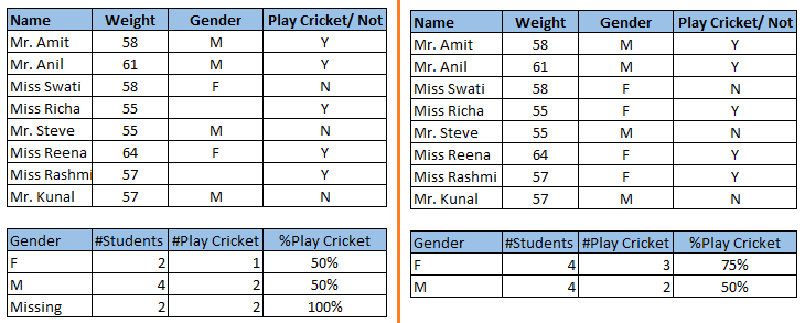
Notice the missing values in the image shown above: In the left scenario, we have not treated missing values. The inference from this data set is that the chances of playing cricket by males is higher than females. On the other hand, if you look at the second table, which shows data after treatment of missing values (based on gender), we can see that females have higher chances of playing cricket compared to males.
Why my data has missing values?
We looked at the importance of treatment of missing values in a dataset. Now, let’s identify the reasons for occurrence of these missing values. They may occur at two stages:
- Data Extraction: It is possible that there are problems with extraction process. In such cases, we should double-check for correct data with data guardians. Some hashing procedures can also be used to make sure data extraction is correct. Errors at data extraction stage are typically easy to find and can be corrected easily as well.
- Data collection: These errors occur at time of data collection and are harder to correct. They can be categorized in four types:
- Missing completely at random: This is a case when the probability of missing variable is same for all observations. For example: respondents of data collection process decide that they will declare their earning after tossing a fair coin. If an head occurs, respondent declares his / her earnings & vice versa. Here each observation has equal chance of missing value.
- Missing at random: This is a case when variable is missing at random and missing ratio varies for different values / level of other input variables. For example: We are collecting data for age and female has higher missing value compare to male.
- Missing that depends on unobserved predictors: This is a case when the missing values are not random and are related to the unobserved input variable. For example: In a medical study, if a particular diagnostic causes discomfort, then there is higher chance of drop out from the study. This missing value is not at random unless we have included “discomfort” as an input variable for all patients.
- Missing that depends on the missing value itself: This is a case when the probability of missing value is directly correlated with missing value itself. For example: People with higher or lower income are likely to provide non-response to their earning.


Comments
Post a Comment