Basic Ensemble Techniques in Machine Learning

 

Introduction
Ensemble models in machine learning operate on a similar idea. They combine the decisions from multiple models to improve the overall performance. This can be achieved in various ways, which you will discover in this article.

Ensembling is nothing but the technique to combine several individual predictive models to come up with the final predictive model. And in this article, we’re going to look at some of the ensembling techniques for both Classification and Regression problems such as Maximum voting, Averaging, Weighted Averaging, and Rank Averaging.

Table of Contents

1. Introduction to Ensemble Learning
2. Basic Ensemble Techniques
   2.1 Max Voting
   2.2 Averaging
   2.3 Weighted Average
3. Advanced Ensemble Techniques
   3.1 Stacking
   3.2 Boosting
   3.3 Bagging
   
4. Algorithms based on Bagging and Boosting
   4.1 Bagging meta-estimator
   4.2 Random Forest
   4.3 AdaBoost
   
   

 

1. Introduction to Ensemble Learning

Let’s understand the concept of ensemble learning with an example. Suppose you are a movie director and you have created a short movie on a very important and interesting topic. Now, you want to take preliminary feedback (ratings) on the movie before making it public. What are the possible ways by which you can do that?

A: You may ask one of your friends to rate the movie for you.
Now it’s entirely possible that the person you have chosen loves you very much and doesn’t want to break your heart by providing a 1-star rating to the horrible work you have created.

B: Another way could be by asking 5 colleagues of yours to rate the movie.
This should provide a better idea of the movie. This method may provide honest ratings for your movie. But a problem still exists. These 5 people may not be “Subject Matter Experts” on the topic of your movie. Sure, they might understand the cinematography, the shots, or the audio, but at the same time may not be the best judges of dark humour.

C: How about asking 50 people to rate the movie?
Some of which can be your friends, some of them can be your colleagues and some may even be total strangers.

2. Simple Ensemble Techniques

In this section, we will look at a few simple but powerful techniques, namely:

1. Max Voting
2. Averaging
3. Weighted Averaging

2.1 Max Voting

The max voting method is generally used for classification problems. In this technique, multiple models are used to make predictions for each data point. The predictions by each model are considered as a ‘vote’. The predictions which we get from the majority of the models are used as the final prediction.

For example, when you asked 5 of your colleagues to rate your movie (out of 5); we’ll assume three of them rated it as 4 while two of them gave it a 5. Since the majority gave a rating of 4, the final rating will be taken as 4. You can consider this as taking the mode of all the predictions.

The result of max voting would be something like this:

Colleague 1	Colleague 2	Colleague 3	Colleague 4	Colleague 5	Final rating
5	4	5	4	4	4

 

Sample Code:

model1 = tree.DecisionTreeClassifier()
model2 = KNeighborsClassifier()
model3= LogisticRegression()

model1.fit(x_train,y_train)
model2.fit(x_train,y_train)
model3.fit(x_train,y_train)

pred1=model1.predict(x_test)
pred2=model2.predict(x_test)
pred3=model3.predict(x_test)

final_pred = np.array([])
for i in range(0,len(x_test)):
    final_pred = np.append(final_pred, mode([pred1[i], pred2[i], pred3[i]]))

Alternatively, you can use “VotingClassifier” module in sklearn as follows:

from sklearn.ensemble import VotingClassifier
model1 = LogisticRegression(random_state=1)
model2 = tree.DecisionTreeClassifier(random_state=1)
model = VotingClassifier(estimators=[('lr', model1), ('dt', model2)], voting='hard')
model.fit(x_train,y_train)
model.score(x_test,y_test)

2.2 Averaging

Similar to the max voting technique, multiple predictions are made for each data point in averaging. In this method, we take an average of predictions from all the models and use it to make the final prediction. Averaging can be used for making predictions in regression problems or while calculating probabilities for classification problems.

For example, in the below case, the averaging method would take the average of all the values.

i.e. (5+4+5+4+4)/5 = 4.4

Colleague 1	Colleague 2	Colleague 3	Colleague 4	Colleague 5	Final rating
5	4	5	4	4	4.4

 

Sample Code:

model1 = tree.DecisionTreeClassifier()
model2 = KNeighborsClassifier()
model3= LogisticRegression()

model1.fit(x_train,y_train)
model2.fit(x_train,y_train)
model3.fit(x_train,y_train)

pred1=model1.predict_proba(x_test)
pred2=model2.predict_proba(x_test)
pred3=model3.predict_proba(x_test)

finalpred=(pred1+pred2+pred3)/3

 

2.3 Weighted Average

This is an extension of the averaging method. All models are assigned different weights defining the importance of each model for prediction. For instance, if two of your colleagues are critics, while others have no prior experience in this field, then the answers by these two friends are given more importance as compared to the other people.

The result is calculated as [(5*0.23) + (4*0.23) + (5*0.18) + (4*0.18) + (4*0.18)] = 4.41.

	Colleague 1	Colleague 2	Colleague 3	Colleague 4	Colleague 5	Final rating
weight	0.23	0.23	0.18	0.18	0.18
rating	5	4	5	4	4	4.41

 

Sample Code:

model1 = tree.DecisionTreeClassifier()
model2 = KNeighborsClassifier()
model3= LogisticRegression()

model1.fit(x_train,y_train)
model2.fit(x_train,y_train)
model3.fit(x_train,y_train)

pred1=model1.predict_proba(x_test)
pred2=model2.predict_proba(x_test)
pred3=model3.predict_proba(x_test)

finalpred=(pred1*0.3+pred2*0.3+pred3*0.4)

 

3. Advanced Ensemble techniques

Now that we have covered the basic ensemble techniques, let’s move on to understanding the advanced techniques.

3.1 Stacking

Stacking is an ensemble learning technique that uses predictions from multiple models (for example decision tree, knn or svm) to build a new model. This model is used for making predictions on the test set. Below is a step-wise explanation for a simple stacked ensemble:

1. The train set is split into 10 parts.
   
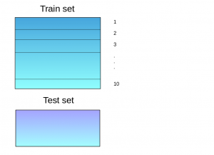
2. A base model (suppose a decision tree) is fitted on 9 parts and predictions are made for the 10th part. This is done for each part of the train set.
   
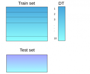
3. The base model (in this case, decision tree) is then fitted on the whole train dataset.
4. Using this model, predictions are made on the test set.
   
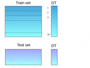
5. Steps 2 to 4 are repeated for another base model (say knn) resulting in another set of predictions for the train set and test set.
   
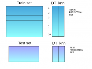
6. The predictions from the train set are used as features to build a new model.
   
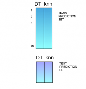
7. This model is used to make final predictions on the test prediction set.

Sample code:

We first define a function to make predictions on n-folds of train and test dataset. This function returns the predictions for train and test for each model.

def Stacking(model,train,y,test,n_fold):
   folds=StratifiedKFold(n_splits=n_fold,random_state=1)
   test_pred=np.empty((test.shape[0],1),float)
   train_pred=np.empty((0,1),float)
   for train_indices,val_indices in folds.split(train,y.values):
      x_train,x_val=train.iloc[train_indices],train.iloc[val_indices]
      y_train,y_val=y.iloc[train_indices],y.iloc[val_indices]

      model.fit(X=x_train,y=y_train)
      train_pred=np.append(train_pred,model.predict(x_val))
      test_pred=np.append(test_pred,model.predict(test))
    return test_pred.reshape(-1,1),train_pred

Now we’ll create two base models – decision tree and knn.

model1 = tree.DecisionTreeClassifier(random_state=1)

test_pred1 ,train_pred1=Stacking(model=model1,n_fold=10, train=x_train,test=x_test,y=y_train)

train_pred1=pd.DataFrame(train_pred1)
test_pred1=pd.DataFrame(test_pred1)

model2 = KNeighborsClassifier()

test_pred2 ,train_pred2=Stacking(model=model2,n_fold=10,train=x_train,test=x_test,y=y_train)

train_pred2=pd.DataFrame(train_pred2)
test_pred2=pd.DataFrame(test_pred2)

Create a third model, logistic regression, on the predictions of the decision tree and knn models.

df = pd.concat([train_pred1, train_pred2], axis=1)
df_test = pd.concat([test_pred1, test_pred2], axis=1)

model = LogisticRegression(random_state=1)
model.fit(df,y_train)
model.score(df_test, y_test)

3.2 Boosting

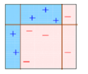
Boosting is a sequential process, where each subsequent model attempts to correct the errors of the previous model. The succeeding models are dependent on the previous model. Let’s understand the way boosting works in the below steps.

1. A subset is created from the original dataset.
2. Initially, all data points are given equal weights.
3. A base model is created on this subset.
4. This model is used to make predictions on the whole dataset.
   
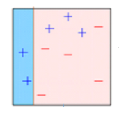
5. Errors are calculated using the actual values and predicted values.
6. The observations which are incorrectly predicted, are given higher weights.
   (Here, the three misclassified blue-plus points will be given higher weights)
7. Another model is created and predictions are made on the dataset.
   (This model tries to correct the errors from the previous model)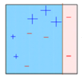
   
8. Similarly, multiple models are created, each correcting the errors of the previous model.
9. The final model (strong learner) is the weighted mean of all the models (weak learners).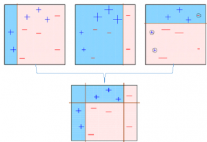Thus, the boosting algorithm combines a number of weak learners to form a strong learner. The individual models would not perform well on the entire dataset, but they work well for some part of the dataset. Thus, each model actually boosts the performance of the ensemble.

3.3 Bagging

The idea behind bagging is combining the results of multiple models (for instance, all decision trees) to get a generalized result. Here’s a question: If you create all the models on the same set of data and combine it, will it be useful? There is a high chance that these models will give the same result since they are getting the same input. So how can we solve this problem? One of the techniques is bootstrapping.

Bootstrapping is a sampling technique in which we create subsets of observations from the original dataset, with replacement. The size of the subsets is the same as the size of the original set.

Bagging (or Bootstrap Aggregating) technique uses these subsets (bags) to get a fair idea of the distribution (complete set). The size of subsets created for bagging may be less than the original set.

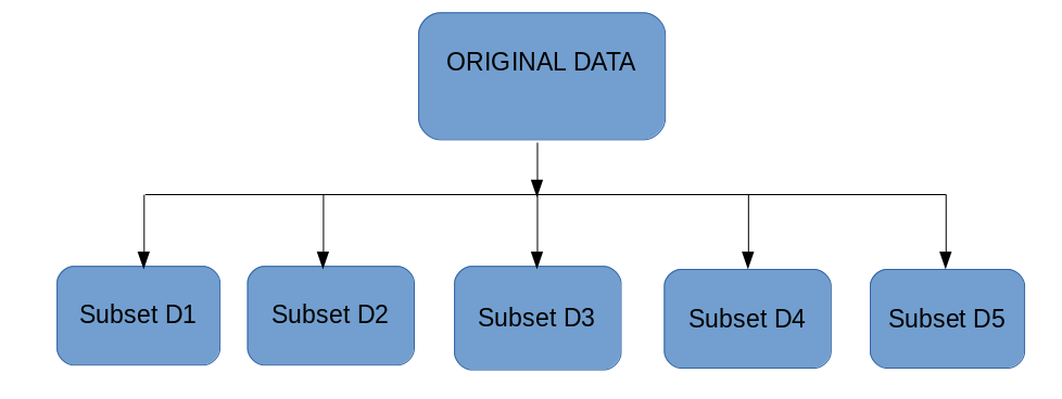
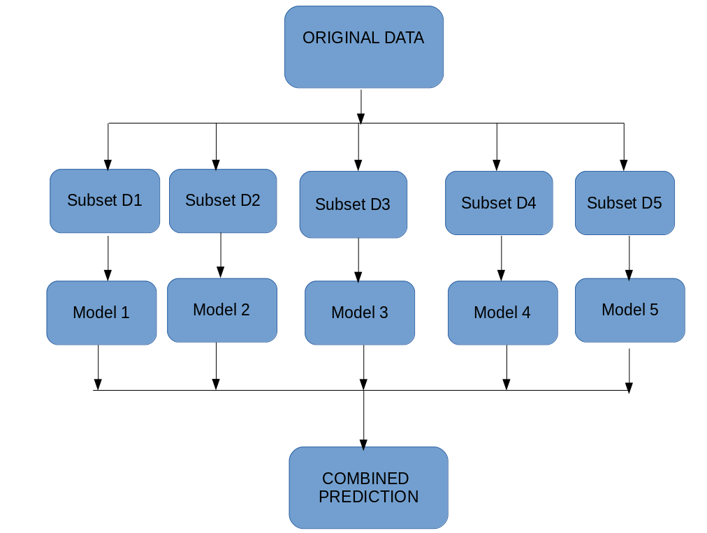
1. Multiple subsets are created from the original dataset, selecting observations with replacement.
2. A base model (weak model) is created on each of these subsets.
3. The models run in parallel and are independent of each other.
4. The final predictions are determined by combining the predictions from all the models.

 

4. Algorithms based on Bagging and Boosting

Bagging and Boosting are two of the most commonly used techniques in machine learning. In this section, we will look at them in detail. Following are the algorithms we will be focusing on:

Bagging algorithms:

• Bagging meta-estimator
• Random forest

Boosting algorithms:

• AdaBoost
• GBM
• XGBM
• Light GBM
• CatBoost

For all the algorithms discussed in this section, we will follow this procedure:

• Introduction to the algorithm
• Sample code
• Parameters

For this article, I have used the Loan Prediction Problem. You can download the dataset from here. Please note that a few code lines (reading the data, splitting into train-test sets, etc.)  will be the same for each algorithm. In order to avoid repetition, I have written the code for the same below, and further discussed only the code for the algorithm.

#importing important packages
import pandas as pd
import numpy as np

#reading the dataset
df=pd.read_csv("/home/user/Desktop/train.csv")

#filling missing values
df['Gender'].fillna('Male', inplace=True)

Similarly, fill values for all the columns. EDA, missing values and outlier treatment has been skipped for the purposes of this article. To understand these topics, you can go through this article: Ultimate guide for Data Exploration in Python using NumPy, Matplotlib and Pandas.

#split dataset into train and test

from sklearn.model_selection import train_test_split
train, test = train_test_split(df, test_size=0.3, random_state=0)

x_train=train.drop('Loan_Status',axis=1)
y_train=train['Loan_Status']

x_test=test.drop('Loan_Status',axis=1)
y_test=test['Loan_Status']

#create dummies
x_train=pd.get_dummies(x_train)
x_test=pd.get_dummies(x_test)

Let’s jump into the bagging and boosting algorithms!

 

4.1 Bagging meta-estimator

Bagging meta-estimator is an ensembling algorithm that can be used for both classification (BaggingClassifier) and regression (BaggingRegressor) problems. It follows the typical bagging technique to make predictions. Following are the steps for the bagging meta-estimator algorithm:

1. Random subsets are created from the original dataset (Bootstrapping).
2. The subset of the dataset includes all features.
3. A user-specified base estimator is fitted on each of these smaller sets.
4. Predictions from each model are combined to get the final result.

Code:

from sklearn.ensemble import BaggingClassifier
from sklearn import tree
model = BaggingClassifier(tree.DecisionTreeClassifier(random_state=1))
model.fit(x_train, y_train)
model.score(x_test,y_test)
0.75135135135135134

Sample code for regression problem:

from sklearn.ensemble import BaggingRegressor
model = BaggingRegressor(tree.DecisionTreeRegressor(random_state=1))
model.fit(x_train, y_train)
model.score(x_test,y_test)

Parameters used in the  algorithms:

• base_estimator:
  • It defines the base estimator to fit on random subsets of the dataset.
  • When nothing is specified, the base estimator is a decision tree.
• n_estimators:
  • It is the number of base estimators to be created.
  • The number of estimators should be carefully tuned as a large number would take a very long time to run, while a very small number might not provide the best results.
• max_samples:
  • This parameter controls the size of the subsets.
  • It is the maximum number of samples to train each base estimator.
• max_features:
  • Controls the number of features to draw from the whole dataset.
  • It defines the maximum number of features required to train each base estimator.
• n_jobs:
  • The number of jobs to run in parallel.
  • Set this value equal to the cores in your system.
  • If -1, the number of jobs is set to the number of cores.

• random_state:
  • It specifies the method of random split. When random state value is same for two models, the random selection is same for both models.
  • This parameter is useful when you want to compare different models.

 

4.2 Random Forest

Random Forest is another ensemble machine learning algorithm that follows the bagging technique. It is an extension of the bagging estimator algorithm. The base estimators in random forest are decision trees. Unlike bagging meta estimator, random forest randomly selects a set of features which are used to decide the best split at each node of the decision tree.

Looking at it step-by-step, this is what a random forest model does:

1. Random subsets are created from the original dataset (bootstrapping).
2. At each node in the decision tree, only a random set of features are considered to decide the best split.
3. A decision tree model is fitted on each of the subsets.
4. The final prediction is calculated by averaging the predictions from all decision trees.

Note: The decision trees in random forest can be built on a subset of data and features. Particularly, the sklearn model of random forest uses all features for decision tree and a subset of features are randomly selected for splitting at each node.